
Predicting Uber Pickups in NYC
SPSS
Introduction
As rideshares are increasingly becoming more popular, it is important to look into the trends of rides based on environmental factors within major cities. Specifically, in New York City, over half of its inhabitants use public transportation on a daily basis and many don’t own a vehicle. Because of this, rideshare services and taxis are the go-to in many situations. With the traffic and weather changes that are present in New York City, knowing how many Ubers are needed on certain days and times is important.
Business Understanding
To optimize their operations in New York City, Uber needs to understand how weather, locations, dates, and times affect the number of rides requested and the peak time designation. Descriptive statistics can identify potential trends in Uber activity in New York City and can help Uber understand how their service is being used in the city. Predictive analytics can help Uber plan for specific times or weather events in certain boroughs.
Data Understanding/Preparation
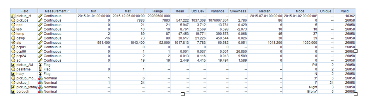
The data was gathered from Kaggle.com. The data has Uber pickups in NYC, with weather, borough, and holidays. The unit of analysis is one hour blocks of time. Pickups were recorded from January 1, 2015 to June 30, 2015 within six boroughs. This dataset contains eighteen variables and has 26,058 rows of data with no missing values. Four variables were derived from the data to further analyze pickup trends-- pickup_month, pickup_AMPM, pickup_t, and pickup_tofday. A data audit and exploratory analysis was done on all eighteen variables to find the distributions, descriptive statistics, and to identify outliers and missing values.
Categorical Variables:
pickup_month: Number of month (1-12)
pickup_AMPM: Whether pick up time was AM or PM
pickup_t: Time of pick up on 24/hr clock
pickup_TofDay: Whether pick up time was Morning (6:00am-12:00pm), Afternoon (12:00pm-6:00pm), or Night (6:00pm-6:00am)
borough: NYC borough (Bronx, Brooklyn, EWR, Manhattan, Queens, Staten Island)
peaktime: derived column based on mean number of pickups in that borough (1 = over average number of pickups, 0 = at or below the mean)
hday: Being a holiday (Y) or not (N)
Continuous Variables:
pickup_dt: Date of pickup
pickups: Number of pickups for the time block
spd: Wind speed in miles/hour
vsb: Visibility in miles to nearest tenth
temp: Temperature in Fahrenheit
dewp: Dewpoint in Fahrenheit
slp: Sea level pressure
pcp01: 1-hour liquid precipitation
pcp06: 6-hour liquid precipitation
pcp24: 24-hour liquid precipitation
sd: Snow depth in inches
Based on exploratory research, we determined which boroughs see the most and least Uber pickup activity and which days and times have the most and least pickup activity. Manhattan had the most total Uber pickups by far. The fewest pickups were at the Newark International Airport (EWR). This is because Uber is not allowed to operate at that airport so pickups from there were either a mistake or conducted without the knowledge of the airport. Of the six months of data included in this study, June had the highest number of pickups (2,814,873). Specifically, the date June 27, 2015 had the most pickups of the six-month period (135,054). 7:00PM was the hour block of time that had the most pickups (1,012,936).


Modeling/Evaluation
Based on predictive analytics, we wanted to determine if the weather, holidays or certain days or times, and location affected the number of pickups or peak time designation in NYC. The specific questions we explored were:
Can blocks of time of Uber activity in NYC be clustered into similar groups?
Are pickups or peak time designations affected by weather? Do certain weather variables affect pickups more than others?
Are pickups or peak time designations affected by holidays?
Are pickups or peak time designations affected by certain days or times?
Are the number of pickups affected by location?
In order to analyze the data, several methods were used. For unsupervised learning, a K-Means cluster analysis was run. For supervised learning, a categorical target variable assessment and a continuous target variable assessment was done. For the categorical target variable (peaktime) assessment, a classification tree and logistic regression were run and for the continuous target variable (pickups) assessment, a regression tree and neural network were run. Models were chosen for their accuracy in predicting the target variables. Linear regression was not used to predict pickups because the model accuracy was lower than the accuracies of the regression tree and neural network.
K-Means Cluster Analysis
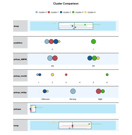
A K-Means cluster analysis was run to identify similarities among records. Understanding groupings among records can help Uber understand which blocks of time can be considered similar in terms of pickups. Five clusters were chosen for this dataset because it is a manageable number for understanding the groupings within the data and can be deployed effectively.
Variables with low predictor importance were removed from the model and the final model was left with ten variables: pickup_month, pickup_t, pickups, peaktime, temp, dewp, pickupAMPM_binary, pickup_tofday_Afternooncat, pickup_tofday_Morningcat, and pickup_tofday_Nightcat. With five clusters, the cluster quality was 0.3, which is a fair quality. An ANOVA was run on the clusters to find out if the variables within each cluster were significantly different from each other. It was found that all of the variables included in the model were important in defining and differentiating the clusters.
The clusters were defined as:
Cluster 1: Late Night (after 12AM) Pickups
Cluster 2: Afternoon Pickups
Cluster 3: High Temperature, High Dew Point, High Number of Pickups
Cluster 4: February Pickups, Low Temperature, Low Dew Point, Medium Number of Pickups
Cluster 5: Medium Temperature, Medium Dew Point, Low Number of Pickups


Classification Tree
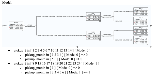
In order to classify records as being peak time or not peak time, a decision tree was built using the CART algorithm. The target variable was peaktime, the input variables were pickup_month, pickup_AMPM, pickup_t, pickup_tofday, spd, vsb, temp, dewp, slp, pcp01, pcp06, pcp24, sd, and hday. The tree was pruned to remove branches that did not improve the predictive ability of the model. After the model was pruned, the variables remaining were pickup_t and pickup_month. The classification tree shows that early morning and afternoon times tend not to be designated as peak times while rush hour times (8-9am) and evening times tend to have higher-than-average requested pickups. Summer months (May and June) tend to have higher-than-average pickups as well.
The accuracy of the model is 0.72 which means the model is accurately predictive. The error rate is 0.28, meaning that 28% of the values were categorized incorrectly. This model shows that the date and time affect whether a block of time is classified as peak time. Weather does not seem to be an important predictor of peak time designation.

If we look at the training data, we can see that if we focus on the top 10%, we will have a 16.588% gain. If we focus on the top 40%, we will have a 66.353% gain and if we focus on the top 50%, we will have a gain of 76.673%. The testing data is very similar to the training data. For the testing data, we can see that if we focus on the top 10%, we will have a 16.547% gain and if we focus on the top 40%, then we will have about an 49.656% gain and if we focus on the top 50%, we will have a gain of 76.117%.
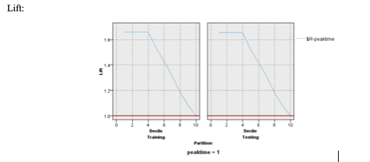

For the testing data, if we focus on the top 10% of our observations, we will have a lift of 1.659 better than random choosing. This continues until the top 40% and then it starts dropping. If we focus on the top 50%, we will have a lift of 1.5327. The training data is fairly similar. If we focus on the top 10% of the training data, lift is 1.6556. This continues until the top 40% and then it starts dropping. If we focus on the top 50%, the lift is 1.5223.
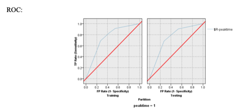
For the ROC chart, we can see the tradeoff between false positives and true positives on the blue line. We can see that if we have a false positive rate of 0.2695, then we have a true positive rate of 0.6885. If we have a false positive rate of 0.4472, then we have a true positive rate of 0.8443. Similarly, for the testing data, if we have a false positive rate of 0.2705 then we have a true positive rate of 0.6849. If we have a false positive rate of 0.4470, then we have a true positive rate of 0.8318.
Logistic Regression
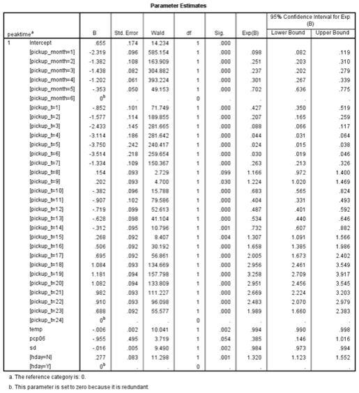
A logistic regression model was built to classify records as being peak time or not peak time. The model was run stepwise to ensure only significant variables were kept. The target variable was peaktime, the final input variables were pickup_month, pickup_t, temp, pcp06, sd, and hday (all p-values less than 0.05). This model shows that the month, time, weather, and holiday affect whether a block of time is classified as peak time.
The accuracy of the model is 0.74 which means the model is accurately predictive. The error rate is 0.26, meaning that 26% of values were categorized incorrectly. This model is best for classifying time blocks as peak time or not. The accuracy is better than the classification tree model and the model is more interpretable.
Equation for peaktime=1:
Logit = -2.319 * [pickup_month=1] + -1.382 * [pickup_month=2] + -1.438 * [pickup_month=3] + -1.202 * [pickup_month=4] + -0.3533 * [pickup_month=5] + -0.8521 * [pickup_t=1] + -1.577 * [pickup_t=2] + -2.433 * [pickup_t=3] + -3.114 * [pickup_t=4] + -3.75 * [pickup_t=5] + -3.514 * [pickup_t=6] + -1.334 * [pickup_t=7] + 0.1539 * [pickup_t=8] + 0.2018 * [pickup_t=9] + -0.3818 * [pickup_t=10] + -0.9066 * [pickup_t=11] + -0.7191 * [pickup_t=12] + -0.6283 * [pickup_t=13] + -0.3124 * [pickup_t=14] + 0.2677 * [pickup_t=15] + 0.5058 * [pickup_t=16] + 0.6954 * [pickup_t=17] + 1.084 * [pickup_t=18] + 1.181 * [pickup_t=19] + 1.082 * [pickup_t=20] + 0.9818 * [pickup_t=21] + 0.9096 * [pickup_t=22] + 0.6876 * [pickup_t=23] + -0.005936 * temp + -0.9554 * pcp06 + -0.01644 * sd + 0.2775 * [hday=N] + 0.6548

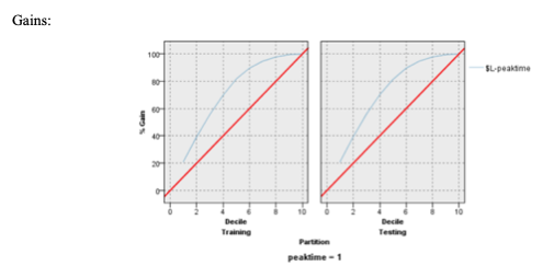
If we look at the training data, we can see that if we focus on the top 10%, we will have a 21.196% gain. If we focus on the top 40%, we will have an 80.748% gain and if we focus on the top 50%, we will have a gain of 55.840%. The testing data is very similar to the training data. For the testing data, we can see that if we focus on the top 10%, we will have a 20.957% gain and if we focus on the top 40%, then we will have about an 70.211% gain and if we focus on the top 50%, we will have a gain of 81.492%.
For the testing data, if we focus on the top 10% of our observations, we will have a lift of 2.1198 better than random choosing. If we focus on the top 30% of our observations, we will have a lift of 1.8616 and we focus on the top 50%, we will have a lift of 1.6338. The training data is fairly similar. If we focus on the top 10% of the training data, lift is 2.0970. If we focus on the top 30%, the lift is 1.8606. If we focus on the top 50%, the lift is 1.6298.
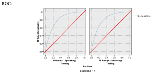
For the ROC chart, we can see the tradeoff between false positives and true positives on the blue line. We can see that if we have a false positive rate of 0.2134 in the training data then we have a true positive rate of 0.6584. If we have a false positive rate of 0.5040, then we have a true positive rate of 0.9250. Similarly, for the testing data, if we have a false positive rate of 0.2748, then we have a true positive rate of 0.7510. If we have a false positive rate of 0.5076, then we have a true positive rate of 0.9223.
Regression Tree
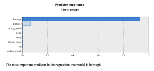
To predict the number of pickups in time blocks, a decision tree was built using the CHAID algorithm. The target variable was pickups, the final input variables were pickup_month, pickup_AMPM, pickup_t, pickup_tofday, borough, slp, temp, and dewp. The strongest predictor variable was borough meaning the location affects the number of pickups most significantly. The month, time, and weather also affect the number of pickups. Within boroughs, higher numbers of pickups are requested at rush hour times and in the evening.
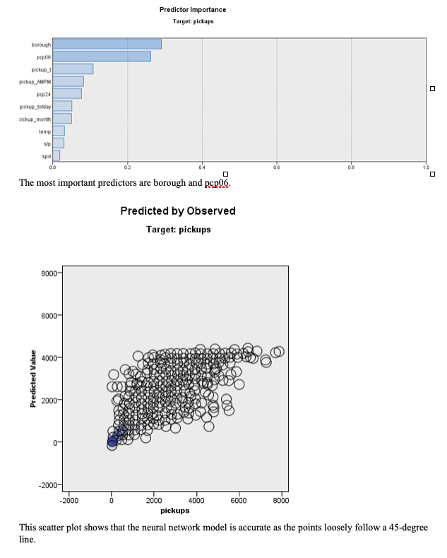
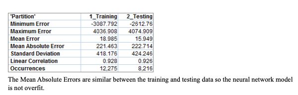
The model is not overfit. The Mean Absolute Error is similar between the training and testing data. Based on the Mean Error, there may be systematic bias in the model. By looking at the scatterplot of actual and estimated number of pickups, the model seems more accurate for smaller numbers of pickups.

Neural Network
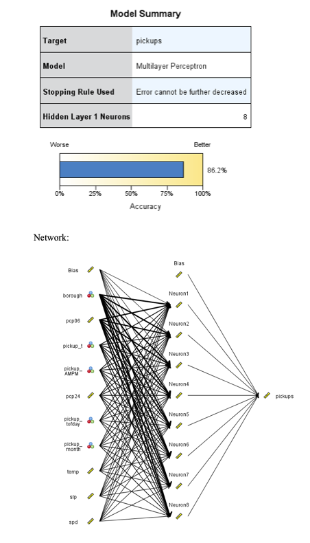
A neural network model was built to predict the number of pickups in time blocks. The target variable was pickups, the input variables were pickup_month, pickup_AMPM, pickup_t, pickup_tofday, borough, spd, temp, slp, pcp24, and pcp06. This model shows that the date, time, location, and weather affect the number of pickups during an hour time block.
The model R2 is 0.862 which is highly predictive. The most important predictor is borough. The model is not overfit to the training data and the Mean Absolute Error is similar between the training and testing data. This model is the best for predicting pickups. Uber maintains a large quantity of data on pickups in different time blocks so the neural network will be able to handle the data better than the regression tree model. While this model is less interpretable than the regression tree, it is accurately predictive so will be useful.
Deployment
For Uber to improve their service, they should consider incorporating predictive analytics into their company's data on a regular basis. They should track pickups, location, time of pickups, and different factors of weather on a daily basis. They should run weekly reports and use multiple predictive models to find trends within their pickups. By doing so, they will increase revenue, gain more customers, normalize their service, and be able to make educated decisions about the future of their company.
Using the clusters, Uber can plan promotional or marketing campaigns for time blocks that are similar to each other. Deploying the logistic regression model (the better of the two categorical target variable models) will allow Uber to use weather forecasts in NYC locations and time to predict if an hour block of time will have higher-than-average requested pickups. Uber will need to track weather forecasts and report on the results of the logistic regression model each day to manage peak times. Deploying the neural network model (the better of the two continuous target variable models) will allow Uber to predict the number of pickups that will be requested based on NYC location, time, and weather. The model will be able to effectively handle the large amount of data Uber collects.
Business Implications
One of the implications of incorporating predictive analytics into Uber’s business is the price of the software, the data analysts, and data collection methods. It has the potential to cost the company a lot of money, but can benefit their company greatly. Another implication is spending a significant amount of money and time on predicting rideshare pickups and not having it benefit their company. Uber can predict pickups, but they can’t force drivers to drive when they want them to. They have very little control over drivers in general. One way to solve that problem is to create monetary incentive for drivers to motivate them to drive when they want them to.
Conclusions
Quality predictive analytics models are necessary for Uber to operate efficiently. Using Uber pickup data combined with weather and location data in New York City from January to June 2015, I was able to build models that clustered and classified records and predicted number of pickups.
My K-Means cluster model shows that records can be grouped into five clusters. Uber can use this to understand how blocks of time are similar in terms of pickups. This may be helpful when planning promotional or marketing campaigns. For example, the clusters show that late-night time blocks are similar to each other but different from afternoon time blocks. Thus, Uber could offer two different promotions targeted towards customers using the service during those times.
The classification models predicted the peak time designation with a good degree of accuracy using date, time, and weather input variables. Peak times are blocks of time where the number of pickups exceeds the mean for that borough. By accurately classifying which times will likely have higher-than-normal Uber requests, Uber can prepare drivers for the increased activity. Uber should deploy the logistic regression model and pull in weather forecasts to create daily reports of expected peak times.
The predictive models built to predict the number of pickups in a block of time were highly accurate using date, time, weather, and location input variables. Uber should deploy the neural network model to utilize the large amount of data Uber collects to predict the number of pickups that can be expected at any given time at locations around New York City. By predicting the number of pickups in an area during a block of time, Uber can determine their expected revenue and the number of drivers needed.